Data types and encodings

Matteo Ceccarello

matteo.ceccarello@unipd.it

Data types

We can classify data types into two broad categories

Ordered
Categorical

Ordered data types

All ordered data has an implicit ordering

Ordinal vs. quantitative
Sequential and diverging
Temporal

Ordinal data types

There is a meaningful ordering, but we cannot do full-fledged arithmetic

Shirt sizes (XS, S, M, L, XL)
Rankings (1st, 2nd, 3rd, 4th, 5th)

Quantitative data

There is a meaningful ordering, and arithmetic operations are supported

Lengths, heights, etc…
Counts
Prices
….

Sequential and diverging data

sequential: where there is a homogeneous range from a minimum to a maximum value

diverging: can be deconstructed into two sequences pointing in opposite directions that meet at a common zero point

Sequential: height of mountains, depth of seas
Diverging: the elevation of points on earth surface; the PH scale (acid to alcaline, with middle point on 7.5)

This distinction will be useful mainly for defining meaningful scales

Temporal data

Time is a complex subject, so temporal data requires special care

Does every year have 365 days?
Does every day have 24 hours?
Does every minute have 60 seconds?
Leap years
Daylight Saving Time
Leap seconds

Dates and times are hard because they have to reconcile two physical phenomena (the rotation of the Earth and its orbit around the sun) with a whole raft of geopolitical phenomena including months, time zones, and DST.

Lubridate

The lubridate package provides a series of facilities to deal with date and times.

It takes care for you of all the gory details of time handling on computers, including time zones, leap years/seconds, daylight saving times, etc…

renv::install("lubridate")
library(lubridate)

It provides three datatypes

date
time
datetime

Creating dates and datetimes

Creating dates

ymd("2019-10-25")

[1] "2019-10-25"

mdy("October 25th, 2019")

[1] "2019-10-25"

dmy("25-Oct-2019")

[1] "2019-10-25"

# On dates that cannot be parsed will return NA
ymd("2019-4r-31")

[1] NA

Creating datetimes

ymd_hms("2019-10-25 08:10:03")

[1] "2019-10-25 08:10:03 UTC"

From components

make_date(2019, 10, 25)

[1] "2019-10-25"

make_datetime(2019, 10, 25, 8, 10, 25)

[1] "2019-10-25 08:10:25 UTC"

With vectorization

dates <- c(
  "October 25th, 2019",
  "October 26th, 2019",
  "Novembber 3rd, 2019",
  "November 4rd, 2019"
)
mdy(dates)

[1] "2019-10-25" "2019-10-26" NA           "2019-11-04"

Bringing proper dates to nycflights13

library(nycflights13)
library(tidyverse)
library(lubridate)

flights |>
  drop_na(dep_delay) |>
  mutate(date = make_date(year, month, day)) |> 
  group_by(date) |>
  summarise(dep_delay = mean(dep_delay)) |> 
  ggplot(aes(x=date, y=dep_delay)) +
    geom_line()

Bringing proper dates to nycflights13

library(nycflights13)
library(tidyverse)
library(lubridate)

flights |>
  drop_na(dep_delay) |>
  mutate(date = make_date(year, month, day)) |> 
  group_by(date, origin) |>
  summarise(dep_delay = mean(dep_delay)) |> 
  ggplot(aes(x=date, y=dep_delay, color=origin)) +
    geom_line()

Bringing proper dates to nycflights13

library(nycflights13)
library(tidyverse)
library(lubridate)

flights |>
  drop_na(dep_delay) |>
  mutate(date = make_date(year, month, day)) |> 
  group_by(date, origin) |>
  summarise(dep_delay = mean(dep_delay)) |> 
  ggplot(aes(x=date, y=dep_delay, color=origin)) +
    geom_line() +
    facet_wrap(vars(origin))

Bringing proper dates to nycflights13

flights |>
  drop_na(dep_delay) |>
  mutate(
    date = make_date(year, month, day),
    weekday = wday(date, label=FALSE), # Gets the day of the week
    weekday_str = wday(date, label=TRUE)
  ) |> 
  group_by(weekday, weekday_str) |>
  summarise(dep_delay = mean(dep_delay)) |> 
  ggplot(aes(x=weekday_str, y=dep_delay)) +
    geom_col(width = 1) +
    coord_polar()

Bringing proper dates to nycflights13

flights |> 
  drop_na(dep_delay) |> 
  mutate(date = make_date(year, month, day)) |> 
  group_by(date, origin) |> 
  summarise(dep_delay = mean(dep_delay)) |> 
  mutate(
    weekday = wday(date, label=TRUE), 
    weeknum = isoweek(date))  |> 
  ggplot(aes(x=weekday, y=weeknum, 
             fill=dep_delay)) +
  geom_tile() +
  scale_fill_continuous(type="viridis") +
  facet_wrap(vars(origin)) +
  theme_bw() +
  theme(legend.position = 'bottom')

Bringing proper dates to nycflights13

flights |> 
  drop_na(dep_delay) |> 
  mutate(date = make_date(year, month, day)) |> 
  group_by(date, origin) |> 
  summarise(dep_delay = mean(dep_delay)) |> 
  mutate(
    weekday = wday(date, label=TRUE), 
    weeknum = isoweek(date))  |> 
  ggplot(aes(x=weekday, y=weeknum, 
             fill=dep_delay, color=dep_delay)) +
  geom_tile() +
  scale_fill_continuous(type="viridis", aesthetics=c("fill","color")) +
  facet_wrap(vars(origin)) +
  coord_polar() +
  theme_void() +
  theme(axis.text.x = element_text(),
        strip.text = element_text(size=14),
        legend.position = 'bottom')

Categorical

Categorical types do not have an implicit ordering.

With categories you can just compare for equality

Apples, organes, bananas, grapes…

You can enforce an explicit ordering when needed

Forcats

This is a tidyverse library that helps with working with categorical data, which in R is called a factor

library(forcats)

Creating factors

You can use the factor function to create factors, which is vectorized

library(gapminder)

mutate(gapminder,
       country = factor(country))

# A tibble: 1,704 x 6
   country     continent  year lifeExp      pop gdpPercap
   <fct>       <fct>     <int>   <dbl>    <int>     <dbl>
 1 Afghanistan Asia       1952    28.8  8425333      779.
 2 Afghanistan Asia       1957    30.3  9240934      821.
 3 Afghanistan Asia       1962    32.0 10267083      853.
 4 Afghanistan Asia       1967    34.0 11537966      836.
 5 Afghanistan Asia       1972    36.1 13079460      740.
 6 Afghanistan Asia       1977    38.4 14880372      786.
 7 Afghanistan Asia       1982    39.9 12881816      978.
 8 Afghanistan Asia       1987    40.8 13867957      852.
 9 Afghanistan Asia       1992    41.7 16317921      649.
10 Afghanistan Asia       1997    41.8 22227415      635.
# i 1,694 more rows

Factors and strings

What is the difference between factors and strings?

Factors can take only a pre-specified number of values

x <- factor(c("a", "b", "c"))
x[4] <- "d"
x

[1] a    b    c    <NA>
Levels: a b c

x <- factor(c("a", "b", "c"), levels = c("a", "b", "c", "d"))
x[4] <- "d"
x

[1] a b c d
Levels: a b c d

You can impose an ordering different than alphabetical to factors.

Reordering factors

gapminder |>
  filter(year==2007) |>
  filter(continent == 'Europe') |> 
  ggplot(aes(x=country, y=gdpPercap)) +
    geom_point() +
    coord_flip()

Reordering factors

gapminder |>
  filter(year==2007) |>
  filter(continent == 'Europe') |> 
  mutate(
    country = fct_reorder(country, gdpPercap)
  ) |> 
  ggplot(aes(x=country, y=gdpPercap)) +
    geom_point() +
    coord_flip()

Reordering factors

gapminder |>
  filter(year==2007) |>
  filter(continent == 'Europe') |> 
  mutate(
    country = fct_reorder(country, desc(gdpPercap))
  ) |> 
  ggplot(aes(x=country, y=gdpPercap)) +
    geom_point() +
    coord_flip()

Aesthetics, geoms, and data

Care must be used when selecting the mapping between attributes and aesthetics, as well as when choosing the geometric objects we use.

Aesthetic types

There are mainly two types of aesthetics

Magnitude aesthetics
Identity aesthetics

Aesthetic types

There are mainly two types of aesthetics

Magnitude aesthetics: ordered data
Identity aesthetics: categorical data

Properties

Expressivenes: what can be encoded by what
Effectiveness: the importance should match the salience of the aesthetic, i.e. its noticeability

When choosing a mapping

Accuracy
Discriminability
Separability
Popout

Accuracy

Given a stimulus how close to the it measurement is the human perceptual judgement
Stevens psychophysical power law [1975]
Be careful with encoding linear information with a non perceptually-linear aesthetic

Accuracy

Discriminability

If you encode data using a particular aesthetic, are the differences between items perceptible to the human as intended?
How many levels can be distinguished?
We should quantify the number of bins that are available in a visual channel

Separability

Popout

Popout, or preattentive processing

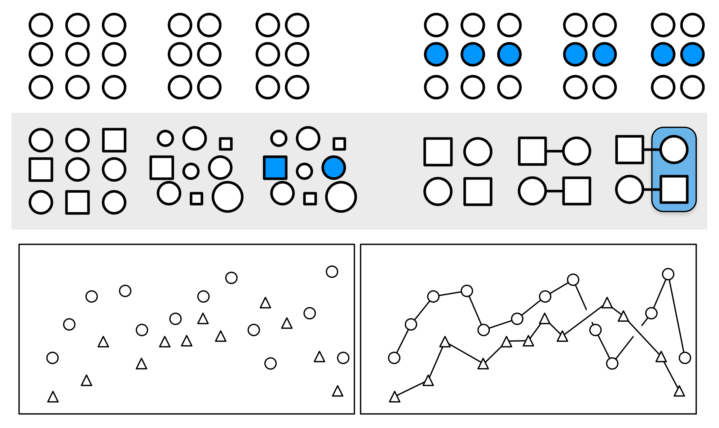
The popout of the color aesthetic is stronger than the one of the shape aesthetic
Using many aesthetics at the same time, for different encodings, might weaken the preattentive effect.
Be very carfeul at representing several variables all at once using different channels: visual conjunctions are often difficult to see (cfr. separability property)
In general, if you want something to stand out, make it different from everything else on prominent (possibly combined) visual channels (e.g. color and size)

Popout, or preattentive processing

Relative vs. absolute judgements

Weber’s Law: our perceptual system is based on relative judgements, not absolute ones. In other terms, our perception is contextual

Relative vs. absolute judgements

Gestalt rules

We look for patterns in what we see:

Proximity: Things that are spatially near to one another seem to be related.
Similarity: Things that look alike seem to be related.
Connection: Things that are visually tied to one another seem to be related.
Continuity: Partially hidden objects are completed into familiar shapes.
Closure: Incomplete shapes are perceived as complete.
Figure and Ground: Visual elements are taken to be either in the foreground or the background.
Common Fate: Elements sharing a direction of movement are perceived as a unit.

Reading list

Munzner: Visualization Analysis and Design, chapters 2 and 5 (in the library)
Ware: Visual thinking for design, chapter 2 (in the library)
Hadley: R for Data Science, chapters 15 and 16